[Decision Tree] Applying decision tree model with R script

How to apply decision tree model and visualizing results

(1) Installing ‘rpart’ package

  install.packages(c('rpart','rpart.plot'))
  library(rpart)
  library(rpart.plot)

(2) Opening the file (n=75)

  sales = read.csv('data/sales.csv')
  head(sales)

##   sales price advert
## 1  73.2  5.69    1.3
## 2  71.8  6.49    2.9
## 3  62.4  5.63    0.8
## 4  67.4  6.22    0.7
## 5  89.3  5.02    1.5
## 6  70.3  6.41    1.3

There three numerical variables: sales, price of products and advertising price. Let’s set sales as dependent variable(y) while the other two are independent variable(x1 and x2).

(3) Using rpart( ), fitting decision tree to the data

  tree_sales = rpart(sales ~ price+advert, data=sales) # '+' mark for multiple independent variables
  tree_sales

## n= 75 
## 
## node), split, n, deviance, yval
##       * denotes terminal node
## 
##  1) root 75 3115.48200 77.37467  
##    2) price>=5.455 46 1108.73800 73.97826  
##      4) price>=6.29 13  183.81080 71.23846 *
##      5) price< 6.29 33  788.90060 75.05758  
##       10) advert< 1.15 10  274.68900 72.29000 *
##       11) advert>=1.15 23  404.31480 76.26087  
##         22) price>=5.84 15  287.23600 75.14000 *
##         23) price< 5.84 8   62.89875 78.36250 *
##    3) price< 5.455 29  634.40830 82.76207  
##      6) advert< 1.4 8  170.44880 78.48750 *
##      7) advert>=1.4 21  262.09810 84.39048  
##       14) price>=5.25 7   72.18000 82.40000 *
##       15) price< 5.25 14  148.31710 85.38571 *

(4) Using rpart.plot( ), visualizing the result

  rpart.plot(tree_sales, cex=1)

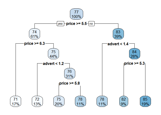
According to the result, the most important criteria is whether price >= 5.5 or not. Recursive partition is kept proceeding with detailed conditions.

Another practice with different data (n=400)

(1) Opening the file

  load('data/admission.RData')
  head(admission)

##   admit gre  gpa rank
## 1     0 380 3.61    3
## 2     1 660 3.67    3
## 3     1 800 4.00    1
## 4     1 640 3.19    4
## 5     0 520 2.93    4
## 6     1 760 3.00    2

    ## admit : admitted or not
    ## gre   : gre score
    ## gpa   : grade point average
    ## rank  : college ranking
  
  nrow(admission)

## [1] 400

(2) Using rpart( ), fitting decision tree to the data

  tree_admit = rpart(admit ~ gre+gpa+rank, data=admission) # '+' mark for multiple independent variables 
  tree_admit

## n= 400 
## 
## node), split, n, loss, yval, (yprob)
##       * denotes terminal node
## 
##   1) root 400 127 0 (0.6825000 0.3175000)  
##     2) gpa< 3.415 208  45 0 (0.7836538 0.2163462)  
##       4) rank=3,4 99  13 0 (0.8686869 0.1313131) *
##       5) rank=1,2 109  32 0 (0.7064220 0.2935780)  
##        10) gre< 730 99  25 0 (0.7474747 0.2525253) *
##        11) gre>=730 10   3 1 (0.3000000 0.7000000) *
##     3) gpa>=3.415 192  82 0 (0.5729167 0.4270833)  
##       6) rank=2,3,4 160  58 0 (0.6375000 0.3625000)  
##        12) rank=3,4 89  27 0 (0.6966292 0.3033708) *
##        13) rank=2 71  31 0 (0.5633803 0.4366197)  
##          26) gpa>=3.495 55  20 0 (0.6363636 0.3636364)  
##            52) gpa< 3.73 26   5 0 (0.8076923 0.1923077) *
##            53) gpa>=3.73 29  14 1 (0.4827586 0.5172414)  
##             106) gre>=690 9   3 0 (0.6666667 0.3333333) *
##             107) gre< 690 20   8 1 (0.4000000 0.6000000) *
##          27) gpa< 3.495 16   5 1 (0.3125000 0.6875000) *
##       7) rank=1 32   8 1 (0.2500000 0.7500000) *

(3) Using rpart.plot( ), visualizing the result

  rpart.plot(tree_admit, cex=1)

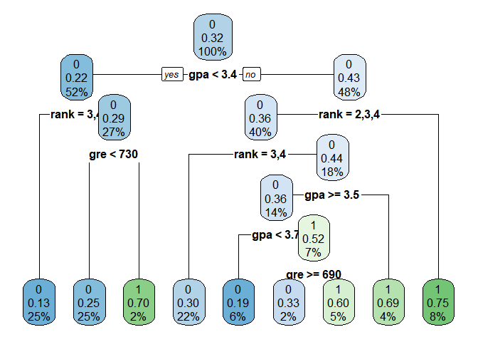
According to the result, the most important criteria is whether gpa<3.4 or not. Recursive partition is kept proceeding with detailed conditions.

Reference

• 패스트 캠퍼스 데이터 분석 입문 올인원 패키지 강의