
[k-NN] Practicing k-Nearest Neighbors classification using cross validation with Python
Understanding k-nearest Neighbors algorithm(k-NN)
- k-NN is one the simplest supervised machine leaning algorithms mostly used for classification, but also for regression.
- In k-NN classification, the input consists of the k closest training examples in dataset, and the output consists of labels of a class. Here, k is a positive integer.
- k-NN stores all available cases and classifies new cases based on a similarity measure.
- k-NN classifies a new data point based on how its neighbors are classified. To be more specific, the new data point is classified by a plurality vote of its neighbors and assigned to the class most common among its k nearest neighbors.
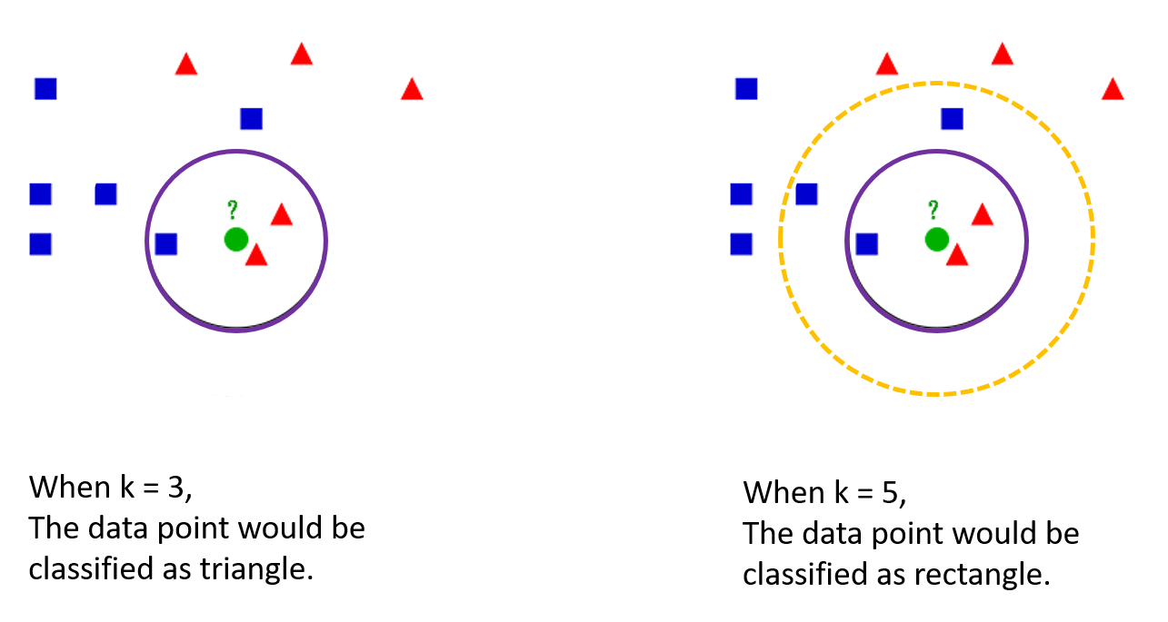
How to decide k ?
-
The optimal k differs from data.
-
When k is too small:
- There would a concern of overfitting.
- Outliers would be greatly affected in classifying a data point.
-
The pattern would not be intuitive.
-
When k is too big:
- There would be a difficulty in classifying data points at the boundaries.
-
When y is categorical:
- In binary classification problems, it is helpful to choose k to be an odd number as this avoids tied votes.
How to calculate distance?
- When there are n of training examples (Xi, Yi), i = 1, …, N, they are arranged by following condition:
- d(X(1), x) ≤ … ≤ d(X(n), x)
- Regarding distance d(a, b):
- When independent variables are categorical: Hamming distance
- When independent variables are continuous: Euclidian distance, Manhattan distance.
[k-NN] Practicing k-Nearest Neighbors classification using cross validation with Python
(1) Importing modules and data
from sklearn import neighbors, datasets
import numpy as np
import matplotlib.pyplot as plt
from matplotlib.colors import ListedColormap
iris = datasets.load_iris()
Data information
print(iris.DESCR)
.. _iris_dataset:

Iris plants dataset
--------------------

**Data Set Characteristics:**

    :Number of Instances: 150 (50 in each of three classes)
    :Number of Attributes: 4 numeric, predictive attributes and the class
    :Attribute Information:
        - sepal length in cm
        - sepal width in cm
        - petal length in cm
        - petal width in cm
        - class:
                - Iris-Setosa
                - Iris-Versicolour
                - Iris-Virginica

    :Summary Statistics:

    ============== ==== ==== ======= ===== ====================
                    Min  Max   Mean    SD   Class Correlation
    ============== ==== ==== ======= ===== ====================
    sepal length:   4.3  7.9   5.84   0.83    0.7826
    sepal width:    2.0  4.4   3.05   0.43   -0.4194
    petal length:   1.0  6.9   3.76   1.76    0.9490  (high!)
    petal width:    0.1  2.5   1.20   0.76    0.9565  (high!)
    ============== ==== ==== ======= ===== ====================

    :Missing Attribute Values: None
    :Class Distribution: 33.3% for each of 3 classes.
    :Creator: R.A. Fisher
    :Donor: Michael Marshall (MARSHALL%PLU@io.arc.nasa.gov)
    :Date: July, 1988

The famous Iris database, first used by Sir R.A. Fisher. The dataset is taken
from Fisher's paper. Note that it's the same as in R, but not as in the UCI
Machine Learning Repository, which has two wrong data points.

This is perhaps the best known database to be found in the
pattern recognition literature.  Fisher's paper is a classic in the field and
is referenced frequently to this day.  (See Duda & Hart, for example.)  The
data set contains 3 classes of 50 instances each, where each class refers to a
type of iris plant.  One class is linearly separable from the other 2; the
latter are NOT linearly separable from each other.

.. topic:: References

   - Fisher, R.A. "The use of multiple measurements in taxonomic problems"
     Annual Eugenics, 7, Part II, 179-188 (1936); also in "Contributions to
     Mathematical Statistics" (John Wiley, NY, 1950).
   - Duda, R.O., & Hart, P.E. (1973) Pattern Classification and Scene Analysis.
     (Q327.D83) John Wiley & Sons.  ISBN 0-471-22361-1.  See page 218.
   - Dasarathy, B.V. (1980) "Nosing Around the Neighborhood: A New System
     Structure and Classification Rule for Recognition in Partially Exposed
     Environments".  IEEE Transactions on Pattern Analysis and Machine
     Intelligence, Vol. PAMI-2, No. 1, 67-71.
   - Gates, G.W. (1972) "The Reduced Nearest Neighbor Rule".  IEEE Transactions
     on Information Theory, May 1972, 431-433.
   - See also: 1988 MLC Proceedings, 54-64.  Cheeseman et al"s AUTOCLASS II
     conceptual clustering system finds 3 classes in the data.
   - Many, many more ...
X = iris.data[:, :2] ## Only taking the first two features
y = iris.target
(2) Finding an optimal ‘k’ using cross-validation
from sklearn.model_selection import cross_val_score
k_range = range(1,100)
k_scores = []

for k in k_range:
    knn = neighbors.KNeighborsClassifier(k)
    scores = cross_val_score(knn, X,y, cv=10, scoring='accuracy')
    k_scores.append(scores.mean())
plt.plot(k_range, k_scores)
plt.xlabel('K-value')
plt.ylabel('Cross-validated accuracy')
plt.show()
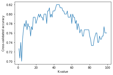
- The accuracy is the highest when K is around 40 to 45 and decrease after that.
- Let’s set k as 45 and do classification with a distance weighted K-NN.
(3) Distance weighted k-NN classification (comparing with a baseline k-NN)
- In this case, the baseline k-NN(weights = ‘uniform’) refers that the all neighbors get an equally weighted “vote” about an observation’s class. On the other hand, weights = ‘distance’ refers to weigh each observation’s “vote” by its distance from the observation we are classifying. (https://chrisalbon.com/machine_learning/nearest_neighbors/k-nearest_neighbors_classifer/)
n_neighbors = 45

h = .02  # step size in the mesh

cmap_light = ListedColormap(['#FFAAAA', '#AAFFAA', '#AAAAFF'])
cmap_bold = ListedColormap(['#FF0000', '#00FF00', '#0000FF'])

for weights in ['uniform', 'distance']:
    clf = neighbors.KNeighborsClassifier(n_neighbors, weights=weights)
    clf.fit(X, y)

    # Plot the decision boundary. For that, we will assign a color to each
    # point in the mesh [x_min, x_max]x[y_min, y_max].
    x_min, x_max = X[:, 0].min() - 1, X[:, 0].max() + 1
    y_min, y_max = X[:, 1].min() - 1, X[:, 1].max() + 1
    xx, yy = np.meshgrid(np.arange(x_min, x_max, h),
                         np.arange(y_min, y_max, h))
    Z = clf.predict(np.c_[xx.ravel(), yy.ravel()])

    # Put the result into a color plot
    Z = Z.reshape(xx.shape)
    plt.figure()
    plt.pcolormesh(xx, yy, Z, cmap=cmap_light)

    # Plot also the training points
    plt.scatter(X[:, 0], X[:, 1], c=y, cmap=cmap_bold,
                edgecolor='k', s=20)
    plt.xlim(xx.min(), xx.max())
    plt.ylim(yy.min(), yy.max())
    plt.title("3-Class classification (k = %i, weights = '%s')"
              % (n_neighbors, weights))

plt.show()
<ipython-input-9-546f7d4814f3>:23: MatplotlibDeprecationWarning: shading='flat' when X and Y have the same dimensions as C is deprecated since 3.3.  Either specify the corners of the quadrilaterals with X and Y, or pass shading='auto', 'nearest' or 'gouraud', or set rcParams['pcolor.shading'].  This will become an error two minor releases later.
  plt.pcolormesh(xx, yy, Z, cmap=cmap_light)
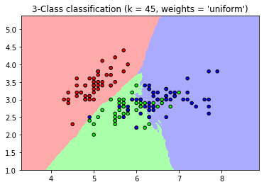
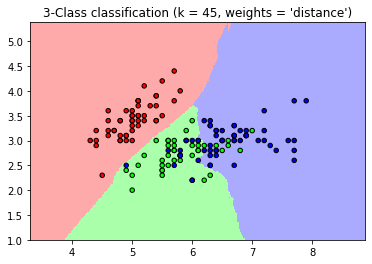
- Compared to the baseline k-NN(weights= ‘uniform’), the distance weighted k-NN shows a clean, intuitive boundary.
(4) Comparing confusion matrices
from sklearn.metrics import confusion_matrix
clf = neighbors.KNeighborsClassifier(n_neighbors=45,weights='uniform')
clf.fit(X,y)
y_pred=clf.predict(X)
confusion_matrix(y,y_pred)
array([[50,  0,  0],
       [ 0, 35, 15],
       [ 1, 10, 39]], dtype=int64)
clf2 = neighbors.KNeighborsClassifier(n_neighbors=45,weights='distance')
clf2.fit(X,y)
y_pred2=clf2.predict(X)
confusion_matrix(y,y_pred2)
array([[50,  0,  0],
       [ 0, 49,  1],
       [ 0, 10, 40]], dtype=int64)
- The distance weighted k-NN has better accuracy than baseline k-NN
More to read
- Nearest Neighbors regression: https://scikit-learn.org/stable/auto_examples/neighbors/plot_regression.html
Reference
- 패스트 캠퍼스 머신러닝과 데이터분석 A-Z 올인원 패키지 Online 강의
- K-Nearest Neighbors Classification: https://chrisalbon.com/machine_learning/nearest_neighbors/k-nearest_neighbors_classifer/
- sklearn.neighbors.KNeighborsClassifier: https://scikit-learn.org/stable/modules/generated/sklearn.neighbors.KNeighborsClassifier.html
- KNN Algorithm Using Python_Simplilearn: https://www.youtube.com/watch?v=4HKqjENq9OU