[Linear Regression] Applying simple and multiple linear regression with R script

How to apply simple linear regression model and interpret results

(1) Opening the file

  heights = read.csv('data/heights.csv')
  head(heights)

##     father      son
## 1 165.2232 151.8368
## 2 160.6574 160.5637
## 3 164.9865 160.8897
## 4 167.0113 159.4926
## 5 155.2886 163.2741
## 6 160.0773 163.1752

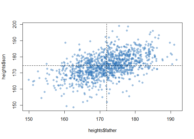
There are two numerical variables: father’s height and son’s height. Let’s set the former as independent variable(x) while the latter is dependent variable(y).

(2) Drawing a scatterplot to visually display the relationship between variables

  plot(heights$father, heights$son, pch=16, col='#3377BB77')+
  abline(v=mean(heights$father), lty=2)+
  abline(h=mean(heights$son),lty=2)

(3) Using lm( ), fitting simple linear regression model to the data

  lm_heights = lm(son ~ father, data=heights)
  summary(lm_heights)

## 
## Call:
## lm(formula = son ~ father, data = heights)
## 
## Residuals:
##      Min       1Q   Median       3Q      Max 
## -22.5480  -3.8466  -0.0201   4.1364  22.7799 
## 
## Coefficients:
##             Estimate Std. Error t value Pr(>|t|)    
## (Intercept) 86.07198    4.65418   18.49   <2e-16 ***
## father       0.51409    0.02705   19.01   <2e-16 ***
## ---
## Signif. codes:  0 '***' 0.001 '**' 0.01 '*' 0.05 '.' 0.1 ' ' 1
## 
## Residual standard error: 6.189 on 1076 degrees of freedom
## Multiple R-squared:  0.2513, Adjusted R-squared:  0.2506 
## F-statistic: 361.2 on 1 and 1076 DF,  p-value: < 2.2e-16

• According to the estimate part from the results, the value of β₀ is 86.07 and β₁ is 0.514 where the simple linear regression equation is Y = β₀ + β₁X
• The coefficient of determination (R2) is 0.25. It means that 25 percent of the variance in the dependent variable(son’s height) can be attributed to the independent variable(dad’s height).

How to apply multiple linear regression model and interpret results

(1) Opening the file

  sales = read.csv('data/sales.csv')
  head(sales)

##   sales price advert
## 1  73.2  5.69    1.3
## 2  71.8  6.49    2.9
## 3  62.4  5.63    0.8
## 4  67.4  6.22    0.7
## 5  89.3  5.02    1.5
## 6  70.3  6.41    1.3

  nrow(sales) 

## [1] 75

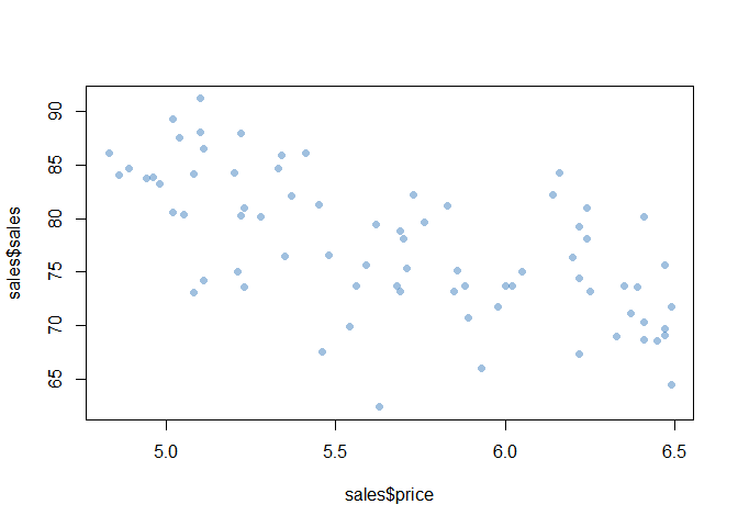
There three numerical variables: sales, price of products and advertising price. Let’s set sales as dependent variable(y) while the other two are independent variable(x1 and x2).

(2) Drawing scatterplots to visually display the relationships between variables

• The scatterplot of price and sales

  plot(sales$price, sales$sales, pch=16, col='#3377BB77')
  

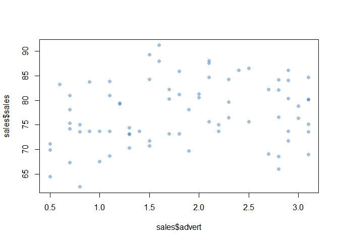
• The scatterplot of advert and sales

  plot(sales$advert, sales$sales, pch=16, col='#3377BB77')
  

(3) Using lm( ), fitting multiple linear regression model to the data

  lm_sales = lm(sales ~ price+advert, data=sales) # '+' mark for multiple independent variables 
  summary(lm_sales)

## 
## Call:
## lm(formula = sales ~ price + advert, data = sales)
## 
## Residuals:
##      Min       1Q   Median       3Q      Max 
## -13.4825  -3.1434  -0.3456   2.8754  11.3049 
## 
## Coefficients:
##             Estimate Std. Error t value Pr(>|t|)    
## (Intercept) 118.9136     6.3516  18.722  < 2e-16 ***
## price        -7.9079     1.0960  -7.215 4.42e-10 ***
## advert        1.8626     0.6832   2.726  0.00804 ** 
## ---
## Signif. codes:  0 '***' 0.001 '**' 0.01 '*' 0.05 '.' 0.1 ' ' 1
## 
## Residual standard error: 4.886 on 72 degrees of freedom
## Multiple R-squared:  0.4483, Adjusted R-squared:  0.4329 
## F-statistic: 29.25 on 2 and 72 DF,  p-value: 5.041e-10

• According to the estimate part from the results, the regression equation is as follows:

  sales = 118.9136 -7.9079sales +1.8626advert

• The coefficient of determination (R2) is 0.4483. It means that about 45 percent of the variance in sales can be attributed to product price and advertising price.

Reference

• 패스트 캠퍼스 데이터 분석 입문 올인원 패키지 강의