[ML] Classification with cilinical data: can we prevent heart failure through data analysis?

About data:

• This analysis includes heart failure clinical records dataset from Kaggle(https://www.kaggle.com/andrewmvd/heart-failure-clinical-data).
• The given CSV file contains such columns below.
  1. age: age of patients
  2. anaemia: decrease of red blood cells or hemoglobin (boolean: 0-normal, 1-anaemia)
  3. creatinine_phosphokinase: level of the CPK enzyme in the blood (mcg/L)
  4. diabetes: if the patient has diabetes (boolean: 0-normal, 1-diabetes)
  5. ejection_fraction: percentage of blood leaving the heart at each contraction (percentage: %)
  6. high_blood_pressure: If the patient has hypertension (boolean: 0-normal, 1-high blood pressure)
  7. platelets: platelets in the blood (kiloplatelets/mL)
  8. serum_creatinine: level of serum creatinine in the blood (mg/dL)
  9. serum_sodium: level of serum sodium in the blood (mEq/L)
  10. sex: sex of the patient (binary: 0-woman, 1-man)
  11. smoking: if the patient smokes or not (boolean: 0-no, 1-yes)
  12. time: follow-up period (days)
  13. DEATH_EVENT: If the patient deceased during the follow-up period (boolean: 0-alive, 1-dead)

Goals of the analysis

• Understanding the form of clinical data
• Applying pandas libary
• Acquring insights through data visualization
• Training models based on Scikit-learn
• Applying classification models and evaluating their performance

---

Step 1. Preparing dataset

import pandas as pd
import numpy as np
import matplotlib.pyplot as plt
import seaborn as sns

1-1. Kaggle API setting

import os

os.environ['KAGGLE_USERNAME']="jisuleeoslo"
os.environ['KAGGLE_KEy']=""

1-2. Downloading data and unzipping data

!kaggle datasets download -d andrewmvd/heart-failure-clinical-data

heart-failure-clinical-data.zip: Skipping, found more recently modified local copy (use --force to force download)

import zipfile
with zipfile.ZipFile("heart-failure-clinical-data.zip","r") as zip_ref:
    zip_ref.extractall()

1-3. Opening the csv file with Pandas library

df = pd.read_csv('heart_failure_clinical_records_dataset.csv')

ls

Step 2. Exploratory Data Analysis using descriptive statistics

2-1. Analyzing columns

df.head(5)

	age	anaemia	creatinine_phosphokinase	diabetes	ejection_fraction	high_blood_pressure	platelets	serum_creatinine	serum_sodium	sex	smoking	time	DEATH_EVENT
0	75.0	0	582	0	20	1	265000.00	1.9	130	1	0	4	1
1	55.0	0	7861	0	38	0	263358.03	1.1	136	1	0	6	1
2	65.0	0	146	0	20	0	162000.00	1.3	129	1	1	7	1
3	50.0	1	111	0	20	0	210000.00	1.9	137	1	0	7	1
4	65.0	1	160	1	20	0	327000.00	2.7	116	0	0	8	1

df.info()

<class 'pandas.core.frame.DataFrame'>
RangeIndex: 299 entries, 0 to 298
Data columns (total 13 columns):
 #   Column                    Non-Null Count  Dtype  
---  ------                    --------------  -----  
 0   age                       299 non-null    float64
 1   anaemia                   299 non-null    int64  
 2   creatinine_phosphokinase  299 non-null    int64  
 3   diabetes                  299 non-null    int64  
 4   ejection_fraction         299 non-null    int64  
 5   high_blood_pressure       299 non-null    int64  
 6   platelets                 299 non-null    float64
 7   serum_creatinine          299 non-null    float64
 8   serum_sodium              299 non-null    int64  
 9   sex                       299 non-null    int64  
 10  smoking                   299 non-null    int64  
 11  time                      299 non-null    int64  
 12  DEATH_EVENT               299 non-null    int64  
dtypes: float64(3), int64(10)
memory usage: 30.5 KB

df.describe()

	age	anaemia	creatinine_phosphokinase	diabetes	ejection_fraction	high_blood_pressure	platelets	serum_creatinine	serum_sodium	sex	smoking	time	DEATH_EVENT
count	299.000000	299.000000	299.000000	299.000000	299.000000	299.000000	299.000000	299.00000	299.000000	299.000000	299.00000	299.000000	299.00000
mean	60.833893	0.431438	581.839465	0.418060	38.083612	0.351171	263358.029264	1.39388	136.625418	0.648829	0.32107	130.260870	0.32107
std	11.894809	0.496107	970.287881	0.494067	11.834841	0.478136	97804.236869	1.03451	4.412477	0.478136	0.46767	77.614208	0.46767
min	40.000000	0.000000	23.000000	0.000000	14.000000	0.000000	25100.000000	0.50000	113.000000	0.000000	0.00000	4.000000	0.00000
25%	51.000000	0.000000	116.500000	0.000000	30.000000	0.000000	212500.000000	0.90000	134.000000	0.000000	0.00000	73.000000	0.00000
50%	60.000000	0.000000	250.000000	0.000000	38.000000	0.000000	262000.000000	1.10000	137.000000	1.000000	0.00000	115.000000	0.00000
75%	70.000000	1.000000	582.000000	1.000000	45.000000	1.000000	303500.000000	1.40000	140.000000	1.000000	1.00000	203.000000	1.00000
max	95.000000	1.000000	7861.000000	1.000000	80.000000	1.000000	850000.000000	9.40000	148.000000	1.000000	1.00000	285.000000	1.00000

Applying df.describe(), one can check:

• Wheter binary data are balanced or imblanced. (For example, the mean of sex is 0.64 and that of smoking is 0.32. This implies there are more data of patients who are men than women. The data include more of non-smokers than smokers.)
• Whether there are extreme outliers
• How is the increase rate of each percentile
• Whether some variables are correlated

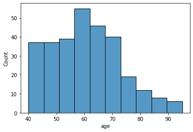
2-2. Drawing histogram on numerical data

import seaborn as sns
sns.histplot(data=df, x='age')

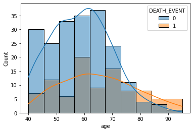
sns.histplot(data=df, x='age', hue='DEATH_EVENT', kde=True)

​
​

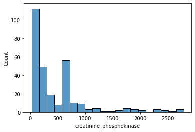
sns.histplot(data=df.loc[df['creatinine_phosphokinase'] < 3000, 'creatinine_phosphokinase'])

​
​

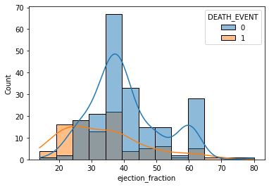
sns.histplot(data=df, x='ejection_fraction', bins=13, hue='DEATH_EVENT', kde=True)

​
​

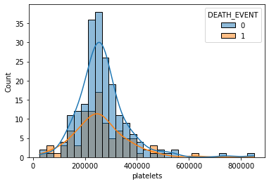
sns.histplot(data=df, x='platelets', hue='DEATH_EVENT', kde=True)

​
​

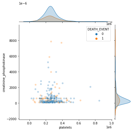
sns.jointplot(x='platelets', y='creatinine_phosphokinase', hue='DEATH_EVENT', data=df, alpha=0.3)

​
​

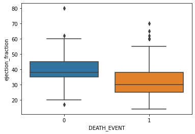
2-3. Drawing boxplot on categorical data

sns.boxplot(x='DEATH_EVENT', y='ejection_fraction', data=df)

​
​

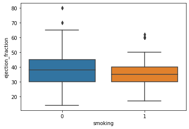
sns.boxplot(x='smoking', y='ejection_fraction', data=df)

​
​

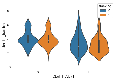
sns.violinplot(x='DEATH_EVENT', y='ejection_fraction', hue='smoking', data=df)

​
​

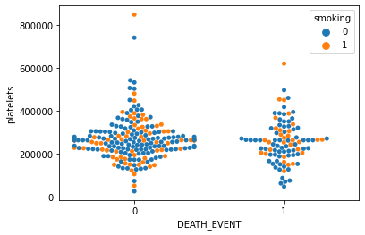
sns.swarmplot(x='DEATH_EVENT', y='platelets', hue='smoking', data=df)

​
​

Step 3. Data pre-processing for modeling

3-1. Feature scaling continous data with StandardScaler

from sklearn.preprocessing import StandardScaler

df.head(5)

	age	anaemia	creatinine_phosphokinase	diabetes	ejection_fraction	high_blood_pressure	platelets	serum_creatinine	serum_sodium	sex	smoking	time	DEATH_EVENT
0	75.0	0	582	0	20	1	265000.00	1.9	130	1	0	4	1
1	55.0	0	7861	0	38	0	263358.03	1.1	136	1	0	6	1
2	65.0	0	146	0	20	0	162000.00	1.3	129	1	1	7	1
3	50.0	1	111	0	20	0	210000.00	1.9	137	1	0	7	1
4	65.0	1	160	1	20	0	327000.00	2.7	116	0	0	8	1

# dividing data into numerical, categorical and output
X_num= df[['age', 'creatinine_phosphokinase', 'ejection_fraction', 'platelets',
       'serum_creatinine', 'serum_sodium', 'time']]
X_cat = df[['anaemia', 'diabetes', 'high_blood_pressure', 'sex', 'smoking']]
y = df['DEATH_EVENT'] 

# Feature scaling continous data and integrating them into numpy array
scaler = StandardScaler()
scaler.fit(X_num)
X_scaled = scaler.transform(X_num)
X_scaled

array([[ 1.19294523e+00,  1.65728387e-04, -1.53055953e+00, ...,
         4.90056987e-01, -1.50403612e+00, -1.62950241e+00],
       [-4.91279276e-01,  7.51463953e+00, -7.07675018e-03, ...,
        -2.84552352e-01, -1.41976151e-01, -1.60369074e+00],
       [ 3.50832977e-01, -4.49938761e-01, -1.53055953e+00, ...,
        -9.09000174e-02, -1.73104612e+00, -1.59078490e+00],
       ...,
       [-1.33339153e+00,  1.52597865e+00,  1.85495776e+00, ...,
        -5.75030855e-01,  3.12043840e-01,  1.90669738e+00],
       [-1.33339153e+00,  1.89039811e+00, -7.07675018e-03, ...,
         5.92615005e-03,  7.66063830e-01,  1.93250906e+00],
       [-9.12335403e-01, -3.98321274e-01,  5.85388775e-01, ...,
         1.99578485e-01, -1.41976151e-01,  1.99703825e+00]])

X_scaled = pd.DataFrame(data=X_scaled, index=X_num.index, columns=X_num.columns)

X = pd.concat([X_scaled, X_cat], axis=1)

X

	age	creatinine_phosphokinase	ejection_fraction	platelets	serum_creatinine	serum_sodium	time	anaemia	diabetes	high_blood_pressure	sex	smoking
0	1.192945	0.000166	-1.530560	1.681648e-02	0.490057	-1.504036	-1.629502	0	0	1	1	0
1	-0.491279	7.514640	-0.007077	7.535660e-09	-0.284552	-0.141976	-1.603691	0	0	0	1	0
2	0.350833	-0.449939	-1.530560	-1.038073e+00	-0.090900	-1.731046	-1.590785	0	0	0	1	1
3	-0.912335	-0.486071	-1.530560	-5.464741e-01	0.490057	0.085034	-1.590785	1	0	0	1	0
4	0.350833	-0.435486	-1.530560	6.517986e-01	1.264666	-4.682176	-1.577879	1	1	0	0	0
...	...	...	...	...	...	...	...	...	...	...	...	...
294	0.098199	-0.537688	-0.007077	-1.109765e+00	-0.284552	1.447094	1.803451	0	1	1	1	1
295	-0.491279	1.278215	-0.007077	6.802472e-02	-0.187726	0.539054	1.816357	0	0	0	0	0
296	-1.333392	1.525979	1.854958	4.902082e+00	-0.575031	0.312044	1.906697	0	1	0	0	0
297	-1.333392	1.890398	-0.007077	-1.263389e+00	0.005926	0.766064	1.932509	0	0	0	1	1
298	-0.912335	-0.398321	0.585389	1.348231e+00	0.199578	-0.141976	1.997038	0	0	0	1	1

299 rows × 12 columns

X.head()

	age	creatinine_phosphokinase	ejection_fraction	platelets	serum_creatinine	serum_sodium	time	anaemia	diabetes	high_blood_pressure	sex	smoking
0	1.192945	0.000166	-1.530560	1.681648e-02	0.490057	-1.504036	-1.629502	0	0	1	1	0
1	-0.491279	7.514640	-0.007077	7.535660e-09	-0.284552	-0.141976	-1.603691	0	0	0	1	0
2	0.350833	-0.449939	-1.530560	-1.038073e+00	-0.090900	-1.731046	-1.590785	0	0	0	1	1
3	-0.912335	-0.486071	-1.530560	-5.464741e-01	0.490057	0.085034	-1.590785	1	0	0	1	0
4	0.350833	-0.435486	-1.530560	6.517986e-01	1.264666	-4.682176	-1.577879	1	1	0	0	0

3-2. Dividing the data into train and test dataset

from sklearn.model_selection import train_test_split

X_train, X_test, y_train, y_test = train_test_split(X, y, test_size=0.33, random_state=1)

X_train

	age	creatinine_phosphokinase	ejection_fraction	platelets	serum_creatinine	serum_sodium	time	anaemia	diabetes	high_blood_pressure	sex	smoking
79	-0.491279	-0.253792	0.585389	0.621074	-0.478205	0.766064	-0.726094	0	0	1	0	0
282	-1.586025	-0.534591	-0.684180	-0.495266	2.329754	-1.958056	1.545334	0	0	0	1	1
297	-1.333392	1.890398	-0.007077	-1.263389	0.005926	0.766064	1.932509	0	0	0	1	1
233	-0.659702	0.129209	-0.007077	0.682524	0.005926	0.085034	1.016195	1	0	0	1	1
106	-0.491279	0.171536	0.585389	-0.003667	-0.090900	0.085034	-0.545412	0	0	0	1	0
...	...	...	...	...	...	...	...	...	...	...	...	...
203	-0.070223	-0.539753	-1.107370	-0.525991	2.039276	-0.141976	0.732266	0	0	1	1	1
255	-0.743913	-0.403483	-0.684180	0.723490	-0.381379	1.220084	1.106535	1	1	1	1	1
72	2.035057	5.471619	-0.260991	-0.208500	-0.381379	-1.050016	-0.751905	0	0	0	1	1
235	1.361368	-0.488136	1.008578	1.460889	-0.284552	0.085034	1.016195	1	0	1	1	0
37	1.782424	0.281997	1.008578	0.590349	-0.381379	1.901114	-1.293951	1	1	1	0	0

200 rows × 12 columns

Step 4. Applying classification models

4-1. Applying Logistic Regression model

from sklearn.linear_model import LogisticRegression

model_lr = LogisticRegression()
model_lr.fit(X_train, y_train)

LogisticRegression()

4-2. Evaluating classification performance of Logistic Regression model

from sklearn.metrics import classification_report

pred = model_lr.predict(X_test)
print(classification_report(y_test, pred))

              precision    recall  f1-score   support

           0       0.86      0.90      0.88        70
           1       0.73      0.66      0.69        29

    accuracy                           0.83        99
   macro avg       0.80      0.78      0.79        99
weighted avg       0.82      0.83      0.83        99

​

4-3. Applying XGBoost model

from xgboost import XGBClassifier

model_xgb = XGBClassifier()
model_xgb.fit(X_train, y_train)

XGBClassifier(base_score=0.5, booster='gbtree', colsample_bylevel=1,
              colsample_bynode=1, colsample_bytree=1, gamma=0, gpu_id=-1,
              importance_type='gain', interaction_constraints='',
              learning_rate=0.300000012, max_delta_step=0, max_depth=6,
              min_child_weight=1, missing=nan, monotone_constraints='()',
              n_estimators=100, n_jobs=8, num_parallel_tree=1, random_state=0,
              reg_alpha=0, reg_lambda=1, scale_pos_weight=1, subsample=1,
              tree_method='exact', validate_parameters=1, verbosity=None)

4-4. Evaluating classification performance of XGBoost model

pred = model_xgb.predict(X_test)
print(classification_report(y_test, pred))

              precision    recall  f1-score   support

           0       0.90      0.91      0.91        70
           1       0.79      0.76      0.77        29

    accuracy                           0.87        99
   macro avg       0.84      0.84      0.84        99
weighted avg       0.87      0.87      0.87        99

​

Too good to be true!

• The accuracy is almost 90%. Maybe there is something missing!

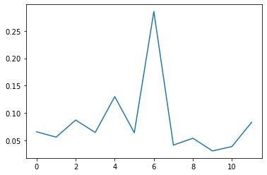
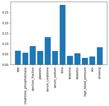
4-5. Finding important features

# What is the important features of XGBClassifier model?
plt.plot(model_xgb.feature_importances_)

plt.bar(X.columns, model_xgb.feature_importances_)
plt.xticks(rotation=90)
plt.show()

​
​

sns.histplot(x='time', data=df, hue='DEATH_EVENT', kde=True)

​
​

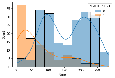
Time as the most important feature?

• Time refers to follow-up period.
• Time strongly depends on the death event.
• Therefore, It could have been better to get rid of ‘time’data.

4-6. Training again without time data

X_num= df[['age', 'creatinine_phosphokinase', 'ejection_fraction', 'platelets',
       'serum_creatinine', 'serum_sodium']]
X_cat = df[['anaemia', 'diabetes', 'high_blood_pressure', 'sex', 'smoking']]
y = df['DEATH_EVENT'] 

scaler = StandardScaler()
scaler.fit(X_num)
X_scaled = scaler.transform(X_num)
X_scaled = pd.DataFrame(data=X_scaled, index=X_num.index, columns=X_num.columns)
X = pd.concat([X_scaled, X_cat], axis=1)

X.head()

	age	creatinine_phosphokinase	ejection_fraction	platelets	serum_creatinine	serum_sodium	anaemia	diabetes	high_blood_pressure	sex	smoking
0	1.192945	0.000166	-1.530560	1.681648e-02	0.490057	-1.504036	0	0	1	1	0
1	-0.491279	7.514640	-0.007077	7.535660e-09	-0.284552	-0.141976	0	0	0	1	0
2	0.350833	-0.449939	-1.530560	-1.038073e+00	-0.090900	-1.731046	0	0	0	1	1
3	-0.912335	-0.486071	-1.530560	-5.464741e-01	0.490057	0.085034	1	0	0	1	0
4	0.350833	-0.435486	-1.530560	6.517986e-01	1.264666	-4.682176	1	1	0	0	0

X_train, X_test, y_train, y_test = train_test_split(X, y, test_size=0.3, random_state=1)

model_lr = LogisticRegression(max_iter=1000)
model_lr.fit(X_train, y_train)

LogisticRegression(max_iter=1000)

pred = model_lr.predict(X_test)
print(classification_report(y_test, pred))

              precision    recall  f1-score   support

           0       0.78      0.92      0.84        64
           1       0.64      0.35      0.45        26

    accuracy                           0.76        90
   macro avg       0.71      0.63      0.65        90
weighted avg       0.74      0.76      0.73        90

​

model_xgb = XGBClassifier()
model_xgb.fit(X_train, y_train)

XGBClassifier(base_score=0.5, booster='gbtree', colsample_bylevel=1,
              colsample_bynode=1, colsample_bytree=1, gamma=0, gpu_id=-1,
              importance_type='gain', interaction_constraints='',
              learning_rate=0.300000012, max_delta_step=0, max_depth=6,
              min_child_weight=1, missing=nan, monotone_constraints='()',
              n_estimators=100, n_jobs=8, num_parallel_tree=1, random_state=0,
              reg_alpha=0, reg_lambda=1, scale_pos_weight=1, subsample=1,
              tree_method='exact', validate_parameters=1, verbosity=None)

pred = model_xgb.predict(X_test)
print(classification_report(y_test, pred))

              precision    recall  f1-score   support

           0       0.81      0.88      0.84        64
           1       0.62      0.50      0.55        26

    accuracy                           0.77        90
   macro avg       0.72      0.69      0.70        90
weighted avg       0.76      0.77      0.76        90

​

plt.bar(X.columns, model_xgb.feature_importances_)
plt.xticks(rotation=90)
plt.show()

​
​

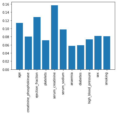
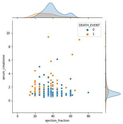
4-7. What is the relationship between the two most important features?

• Serum_creatinine as the most important feature.
• Ejection_fraction as the second important feature.

sns.jointplot(x='ejection_fraction', y='serum_creatinine',hue='DEATH_EVENT',data=df)

​
​

Step 5. In-depth analysis on the learning results

5-1. Idetifying Precision-Recall curve

from sklearn.metrics import plot_precision_recall_curve

plot_precision_recall_curve(model_lr, X_test, y_test)

​
​

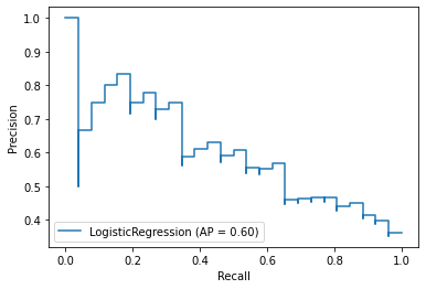
plot_precision_recall_curve(model_xgb, X_test, y_test)

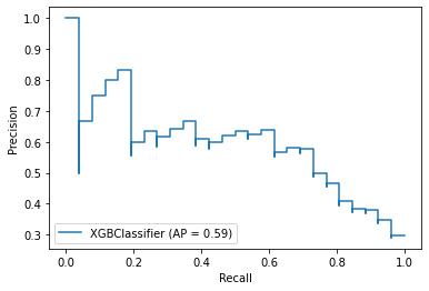
 fig = plt.figure()
 ax = fig.gca()
 plot_precision_recall_curve(model_lr, X_test, y_test,ax=ax)
 plot_precision_recall_curve(model_xgb, X_test, y_test,ax=ax)

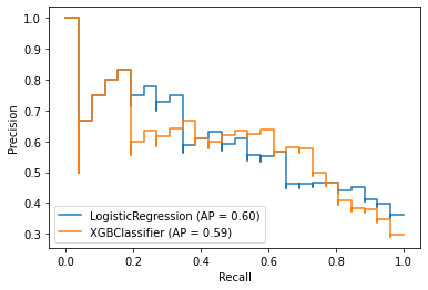
P*R curve implies XGBClassifier yielded better performance on the data

• The closer to 1, the better performance.

5-2. Identifying ROC curve

from sklearn.metrics import plot_roc_curve

fig = plt.figure()
ax = fig.gca()
plot_roc_curve(model_lr, X_test, y_test,ax=ax)
plot_roc_curve(model_xgb, X_test, y_test,ax=ax)
plt.show()

​
​

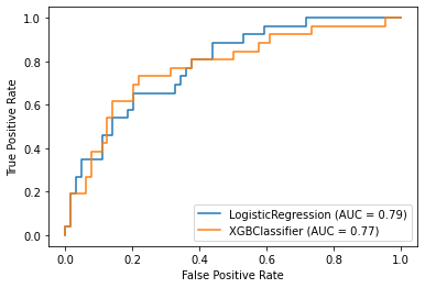
ROC curve implies LogisticRegression yielded better performance on the data

• The faster reaching 1 while keeping low FPS, the better performance.
• The higher Area Under Cover(AUC), the better performance.
• In result, it is difficult to say which model is better than the other.