
[Decision Tree] Experimenting and visualizing classification and regression trees with different depths
1. Decision Classification Tree
(1) Importing modules and data(iris data)
from sklearn.datasets import load_iris
from sklearn import tree
from os import system
system("pip install graphviz")
0
import graphviz
iris=load_iris()
iris.feature_names
['sepal length (cm)',
 'sepal width (cm)',
 'petal length (cm)',
 'petal width (cm)']
iris.target_names
array(['setosa', 'versicolor', 'virginica'], dtype='<U10')
(2) Splitting train dataset and test dataset
from sklearn.model_selection import train_test_split
X_train, X_test, y_train, y_test = train_test_split(iris.data,iris.target, stratify=iris.target,random_state=123)
(3) Making a classificaion decision tree model and comparing accuracy scores with different depths
from sklearn.metrics  import accuracy_score
from sklearn.metrics import confusion_matrix
def compare_depth(max_depth):
    clf=tree.DecisionTreeClassifier(criterion='gini', max_depth=max_depth, random_state=1)
    clf=clf.fit(X_train, y_train)

    y_train_pred = clf.predict(X_train)
    y_test_pred = clf.predict(X_test)

    print(accuracy_score(y_train, y_train_pred))
    print(confusion_matrix(y_train, y_train_pred))
    print(accuracy_score(y_test, y_test_pred))
    print(confusion_matrix(y_test, y_test_pred))
compare_depth(3)
0.9642857142857143
[[38  0  0]
 [ 0 36  1]
 [ 0  3 34]]
0.9210526315789473
[[12  0  0]
 [ 0 12  1]
 [ 0  2 11]]
compare_depth(5)
0.9910714285714286
[[38  0  0]
 [ 0 37  0]
 [ 0  1 36]]
0.9736842105263158
[[12  0  0]
 [ 0 12  1]
 [ 0  0 13]]
compare_depth(7)
1.0
[[38  0  0]
 [ 0 37  0]
 [ 0  0 37]]
0.9736842105263158
[[12  0  0]
 [ 0 12  1]
 [ 0  0 13]]
As it is seen, I made a function for comparing accuracy scores with a different scale of depth. The more depth, the better accuracy yields for train set. This means that the model can explain train data better as it learns data more in details. Yet, when I compared the model with its depth 5 and 7, the accuracy of test dataset was not improved while that of trainset increased up to 100%. It implies that overfitting has occurred between depth = 5 to 7.
(4) Visualizing classification trees
In the beginning, each class has the same or similar number of sample : setosa(38), versicolor(37), virginica(37). Value implies that how many samples belong to each class.
decisiontree_comparision(3)

decisiontree_comparision(5)

decisiontree_comparision(7)

Among above three, to alleviate the overfitting problem, I would choose the second classification decision tree where the tree depth is 5.
2. Decision regression tree
(1) Importing modules and making random data
import numpy as np
from sklearn.tree import DecisionTreeRegressor
import matplotlib.pyplot as plt

rng = np.random.RandomState(1)
X = np.sort(5 * rng.rand(80, 1), axis=0)
y = np.sin(X).ravel()
y[::5] += 3 * (0.5 - rng.rand(16))
(2) Making regression trees with different depths
regr1=tree.DecisionTreeRegressor(max_depth=2)
regr2=tree.DecisionTreeRegressor(max_depth=5)
regr1.fit(X,y)
regr2.fit(X,y)
DecisionTreeRegressor(max_depth=5)
y_1=regr1.predict(X)
y_2=regr2.predict(X)
from sklearn.metrics import mean_squared_error
print(mean_squared_error(y, y_1))
0.12967126328231798
print(mean_squared_error(y, y_2))
0.025236948989861896
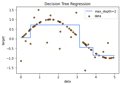
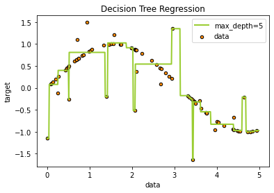
The MSE is smaller when the depth=5 than the depth = 2.
(3) Visualizing how correct regression trees can predict the data with different settings of the depth
X_test=np.arange(0.0,5.0,0.01)[:,np.newaxis]

y_pred_1=regr1.predict(X_test)
y_pred_2=regr2.predict(X_test)
The figure below shows when the tree depth is 2 while the next one shows when the depth is 5
plt.figure()
plt.scatter(X, y, s=20, edgecolor="black", c="darkorange", label="data")
plt.plot(X_test, y_pred_1, color="cornflowerblue", label="max_depth=2", linewidth=2)

plt.xlabel("data")
plt.ylabel("target")
plt.title("Decision Tree Regression")
plt.legend()
plt.show()
plt.figure()
plt.scatter(X, y, s=20, edgecolor="black", c="darkorange", label="data")
plt.plot(X_test, y_pred_2, color="yellowgreen", label="max_depth=5", linewidth=2)

plt.xlabel("data")
plt.ylabel("target")
plt.title("Decision Tree Regression")
plt.legend()
plt.show()
### Plottingn to see the difference when the tree depth is 2 and 5

plt.figure()
plt.scatter(X, y, s=20, edgecolor="black",
            c="darkorange", label="data")
plt.plot(X_test, y_pred_1, color="cornflowerblue",
         label="max_depth=2", linewidth=2)
plt.plot(X_test, y_pred_2, color="yellowgreen", label="max_depth=5", linewidth=2)
plt.xlabel("data")
plt.ylabel("target")
plt.title("Decision Tree Regression")
plt.legend()
plt.show()
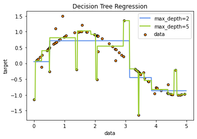
The regression model with depth=2 could find a general trend, while the one with depth=5 could predict more in details. However, the latter might react too sensitive to outliers.
(4) Visualizing regression trees
reg_tree1 = tree.export_graphviz(regr1, out_file=None,
                                filled=True, rounded=True,
                                special_characters=True)
g_reg_tree1 = graphviz.Source(reg_tree1)
g_reg_tree1

reg_tree2 = tree.export_graphviz(regr2, out_file=None,
                                filled=True, rounded=True,
                                special_characters=True)
g_reg_tree2 = graphviz.Source(reg_tree2)
g_reg_tree2

Each graph shows regression trees when its depth is 2 and 5. In the regression trees, value refers to a representative value of samples(for instance, the mean of samples).
Reference
- Scikit-learn: https://scikit-learn.org/stable/auto_examples/tree/plot_tree_regression.html
- 세종대*최유경 교수 9주차 의사결정나무 Part4(유튜브 강의): https://www.youtube.com/watch?v=z683uUHlDeM
- 패스트 캠퍼스 머신러닝과 데이터분석 A-Z 올인원 패키지 Online 강의