[R] Practicing linear regression and decision tree with insurance cost data

Practicing linear regression and decision tree with insurance cost data(from Kaggle)

(1) Downloading the data

Medical Cost Personal Datasets : https://www.kaggle.com/mirichoi0218/insurance

(2) Opening the downloaded csv file

  insurance = read.csv('data/insurance.csv')

(3) Using summary( ), to get descriptive statistics

  summary(insurance)

##       age            sex                 bmi           children    
##  Min.   :18.00   Length:1338        Min.   :15.96   Min.   :0.000  
##  1st Qu.:27.00   Class :character   1st Qu.:26.30   1st Qu.:0.000  
##  Median :39.00   Mode  :character   Median :30.40   Median :1.000  
##  Mean   :39.21                      Mean   :30.66   Mean   :1.095  
##  3rd Qu.:51.00                      3rd Qu.:34.69   3rd Qu.:2.000  
##  Max.   :64.00                      Max.   :53.13   Max.   :5.000  
##     smoker             region             charges     
##  Length:1338        Length:1338        Min.   : 1122  
##  Class :character   Class :character   1st Qu.: 4740  
##  Mode  :character   Mode  :character   Median : 9382  
##                                        Mean   :13270  
##                                        3rd Qu.:16640  
##                                        Max.   :63770

• There are four numerical data: age, BMI, children and charges.
• There are three categorical data: sex, smoker and region.

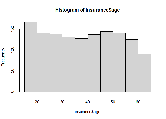
(4) Making histograms with numerical data and tables with categorical data

  hist(insurance$age)

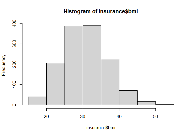
  hist(insurance$bmi)

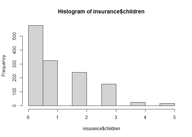
  hist(insurance$children)

  table(insurance$sex)

## 
## female   male 
##    662    676

  table(insurance$smoker)

## 
##   no  yes 
## 1064  274

  table(insurance$region)

## 
## northeast northwest southeast southwest 
##       324       325       364       325

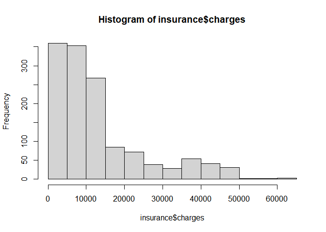
(5) Numerical data - making a scatterplot and calculating correlation coefficient between BMI and charges

  plot(insurance$bmi, insurance$charges, pch=16)

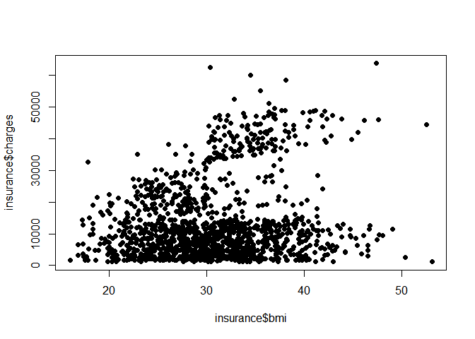
cor(insurance$bmi, insurance$charges)

## [1] 0.198341

• A weak and suspicious positive correlation is found. This alone cannot guarantee us very much about the correlation.

(6) Categorical data - making boxplots of charges by regions, and calculating average charges by regions

  boxplot(charges ~ region, data=insurance)

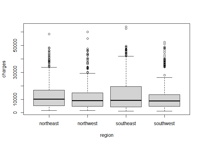
  aggregate(charges ~ region, data=insurance, mean)

##      region  charges
## 1 northeast 13406.38
## 2 northwest 12417.58
## 3 southeast 14735.41
## 4 southwest 12346.94

• The average charges in southeast region is higher than the others.
• In the boxplot, the median values of insurance charges in each region look pretty much similar, yet the top 50 percent of insurance charges in southeast are more expensive than those of the others.

(7) Applying multiple linear regression when the variable of interest variable charges and the others are explanatory variables

  lm_ins = lm(charges ~ ., data=insurance)
  summary(lm_ins)

## 
## Call:
## lm(formula = charges ~ ., data = insurance)
## 
## Residuals:
##      Min       1Q   Median       3Q      Max 
## -11304.9  -2848.1   -982.1   1393.9  29992.8 
## 
## Coefficients:
##                 Estimate Std. Error t value Pr(>|t|)    
## (Intercept)     -11938.5      987.8 -12.086  < 2e-16 ***
## age                256.9       11.9  21.587  < 2e-16 ***
## sexmale           -131.3      332.9  -0.394 0.693348    
## bmi                339.2       28.6  11.860  < 2e-16 ***
## children           475.5      137.8   3.451 0.000577 ***
## smokeryes        23848.5      413.1  57.723  < 2e-16 ***
## regionnorthwest   -353.0      476.3  -0.741 0.458769    
## regionsoutheast  -1035.0      478.7  -2.162 0.030782 *  
## regionsouthwest   -960.0      477.9  -2.009 0.044765 *  
## ---
## Signif. codes:  0 '***' 0.001 '**' 0.01 '*' 0.05 '.' 0.1 ' ' 1
## 
## Residual standard error: 6062 on 1329 degrees of freedom
## Multiple R-squared:  0.7509, Adjusted R-squared:  0.7494 
## F-statistic: 500.8 on 8 and 1329 DF,  p-value: < 2.2e-16

• In the result, for example, when every one year increase in age, the model predicts an increase of 256.9 dollars.
• Under the same conditions but when a patient is a male, the model predicts a decrease of 131.3 dollars.

(8) Applying decision tree when the variable of interest variable charges and the others are explanatory variables

  library(rpart)
  tree_ins = rpart(charges ~ ., data=insurance)
  tree_ins

## n= 1338 
## 
## node), split, n, deviance, yval
##       * denotes terminal node
## 
## 1) root 1338 196074200000 13270.420  
##   2) smoker=no 1064  38188720000  8434.268  
##     4) age< 42.5 596  13198540000  5398.850 *
##     5) age>=42.5 468  12505450000 12299.890 *
##   3) smoker=yes 274  36365600000 32050.230  
##     6) bmi< 30.01 130   3286655000 21369.220 *
##     7) bmi>=30.01 144   4859010000 41692.810 *

  library(rpart.plot)
  rpart.plot(tree_ins)

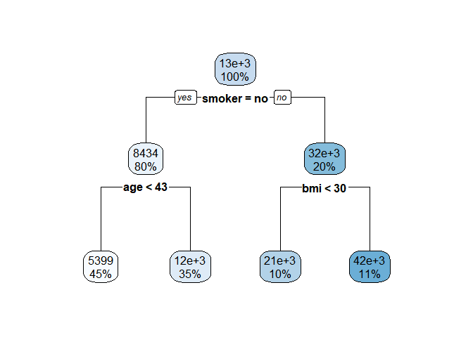
• Depending on a patient’s smoking status, the data is divided into 8: 2 with a large difference in insurance costs. Smokers pay a lot more than non smokers, and whose BMI level is over 30(falling within the obesity range) pay more than the rest of the smokers.
• Meanwhile non-smokers have difference in insurance costs depending on whether they are over 43 years or not.

Reference

• 패스트 캠퍼스 데이터 분석 입문 올인원 패키지 강의