An explanation simple linear regression with R script

1. How to calculate regression coefficient in simple linear regression?

• In simple linear regression a linear function is used to explain the relationship between one independent variable(x) and a dependent variable(y) as accurate as possible, and predict unseen dependent values when certain independent values are given. The independent variable is single and continuous”

• The formula of simple linear regression is Y = β₀  + β₁X when X is a given value of an independent variable, β₀ and β₁ are regression coefficient, and Y is a predicting value of a dependent variable.

• The most used method for calculating regression coefficient is least squares method.

  • 

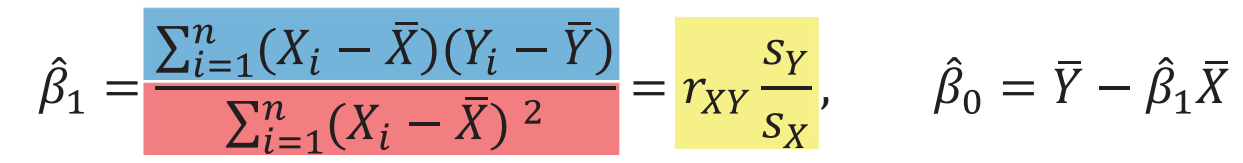
    X͞ is the average of X_i and Y͞ is the average of Y_i

    r_XY is the correlation coefficient between X and Y

    S_X and S_Y is the standard deviation of X and Y

2. R script for understanding simple linear regression

• When data include 1,078 samples of father(X)-son(Y)’s heights, following codes are to draw trend lines representing the averages of X and Y and find a linear function by calculating regression coefficient to make a prediction.

(1) Importing data

heights = read.csv('data/heights.csv')
head(heights)

##     father      son
## 1 165.2232 151.8368
## 2 160.6574 160.5637
## 3 164.9865 160.8897
## 4 167.0113 159.4926
## 5 155.2886 163.2741
## 6 160.0773 163.1752

tail(heights)

##        father      son
## 1073 171.9747 151.9350
## 1074 170.1719 179.7109
## 1075 181.1828 173.4001
## 1076 182.3292 176.0370
## 1077 179.6755 176.0271
## 1078 178.5775 170.2181

(2) Drawing a scatterplot and trend lines

plot(heights, pch=16, col='#3377BB77')
abline(v=mean(heights$father), lty=2)
abline(h=mean(heights$son),lty=2)

(3) Calculating regression coefficient

r_xy = cor(heights$father, heights$son)
r_xy

## [1] 0.5013383

sd_x = sd(heights$father)
sd_y = sd(heights$son)

b1 = r_xy/sd_x*sd_y
b1

## [1] 0.514093

b0 = mean(heights$son) - b1*mean(heights$father)
b0

## [1] 86.07198

plot(heights, pch=16, col='#3377BB77')
abline(v=mean(heights$father), lty=2)
abline(h=mean(heights$son),lty=2)
abline(a=b0, b=b1, col='red', lwd=2)

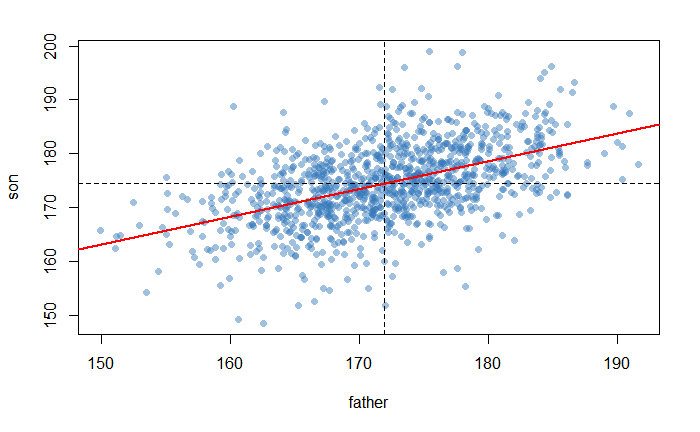
The red line represents the relationship between dad-son’s heights

(4) Prediction applying the given regression coefficient

b0 + b1*175 #When dad's height is 175

## [1] 176.0383

b0 + b1*190 #When dad's height is 190

## [1] 183.7497

Reference

• 패스트캠퍼스 데이터 분석 입문 올인원 패키지 강의